

Light Scattering at Sea
Published: 9 July 2013
Editor’s note: Ernie Lewis, principal investigator for the Marine ARM GPCI Investigations of Clouds (MAGIC) field campaign, introduces us to some MAGIC participants.
In the last update I introduced some MAGIC people, including two college students, Danielle and Michelle, who are working with me on MAGIC data. Another student, Sarah, who will be a senior at a local high school this fall, is also working on MAGIC data with me this summer. As I noted in the last update, I’ve given them a lot to do this summer besides their projects: I require that they attend all seminars in the department, and I gave them a list of nearly a dozen scientists in the department with whom they should speak. I feel this is important so they can be exposed to a wide range of scientific topics and viewpoints. Every day they do the weather, and I ask them if they looked at the clouds on the way in to work. They also have atmospheric questions I’ve given them to think about, like “How big is a cloud drop?” or “If atmospheric CO2 continues to increase, will we run out of oxygen?”
Each of these students is great to work with: they’re smart, very hard-working, and easy to get along with; who could ask for anything more! I asked each of them to write something for these updates, and they agreed to do so. Michelle volunteered to go first; her contribution follows.
***
When Ernie first asked me if I could write a little bit about what I’ve been working on to include in his next update, I initially panicked. Like I tell my parents when they ask me what I did at work today, “I haven’t made a lot of progress, but I’ve gotten a lot done.” As one can imagine, working with data coming from instruments on a moving ship in the middle of the Pacific Ocean is a lot different than processing numbers that have been carefully designed by my professors to give expected results. Although raw data is not as nice to work with, processing and analyzing real world data has been extremely rewarding.
Part of the reason MAGIC is such an important initiative is because modeling the Earth’s climate is incredibly complex and difficult. Gathering as much information as possible about the innumerable factors that influence climate is essential to improving global models and better understanding our atmosphere. MAGIC investigators are especially interested in the role that aerosols, small particles suspended in the air, play in shaping climate. To put things in perspective, here at the lab, typical aerosol concentrations range from 600 to 1000 particles per cubic centimeter. On the way from LA to Hawaii, over the ocean, the concentration drops significantly to about 100-200 particles per cubic centimeter. Understanding how aerosols affect climate is complicated by the numerous and contradictory ways in which aerosols affect the Earth’s energy balance.
As Ernie mentioned in the last update, my main project for the summer is to look at two instruments measuring aerosol properties on Spirit as it travels across the Pacific Ocean and compare the two sets of data to see if the measurements agree. The two instruments in question are the UHSAS (ultra-high sensitivity aerosol spectrometer) and the nephelometer. The UHSAS measures the number and size of aerosol particles in the air. It can detect particles with a diameter as small as 55 nanometers, which is roughly 1/1000th the diameter of a human hair. The nephelometer is an instrument that measures how much red, blue, and green light is scattered by these aerosol particles.
By using information about the size and concentration of aerosol particles from the UHSAS, we can predict how much light scattering should be measured by the nephelometer. Results from this comparison can help us to identify inaccuracies in the data from one of the instruments. Furthermore, if the calculated scattering agrees with the measured scattering, it is an indication that the instruments might be working properly and providing reliable data.
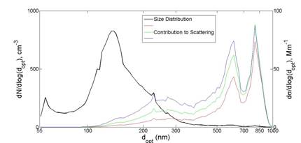
How light interacts with aerosol particles is affected by variations in particle size and composition. The UHSAS counts how many particles flow through it and categorizes them into 99 different size bins. Using this data, one can construct a size distribution (black line), which shows how many particles are in each size bin. From the size distribution, the expected amount of scattering can be calculated for red light (700 nm wavelength), green light (550 nm wavelength), and blue light (450 nm wavelength). The estimated scattering for the different wavelengths of light is represented by the red, green, and blue lines on the graph. As you can see, blue light scatters the most and red light scatters the least for smaller particles. This is the same reason why the sky is blue during the day, and turns red at sunset. On a clear day the sky is blue because blue light scatters off of molecules more than red light does. In the evening, light from the setting sun has to pass through more of the atmosphere to reach the Earth’s surface than it does in the middle of the day when the sun is high in the sky. As the light from the sun travels through the atmosphere, even more blue light is scattered away, making the red and orange light visible.
The graph shows that although most of the particles are between 100 and 250 nanometers in diameter, the particles that account for a bulk of the scattering are larger, between 500–900 nanometers in diameter. This tells us that in terms of light scattering, a few bigger particles play a much larger role than a bunch of tiny particles. This has large implications in terms of climate modeling in that larger sea-salt particles suspended over the Pacific Ocean will scatter light differently than the tiny anthropogenic pollution particles near L.A.
***
Thanks, Michelle! You’ve set a high bar for the others.
Ernie Lewis
The ARM Climate Research Facility is a DOE Office of Science user facility. The ARM Facility is operated by nine DOE national laboratories, including .
Follow Us:


Keep up with the Atmospheric Observer
Updates on ARM news, events, and opportunities delivered to your inbox
ARM User Profile
ARM welcomes users from all institutions and nations. A free ARM user account is needed to access ARM data.